Imp needed a relational database that is simple enough to experiment with but fast enough to power real applications.
Relational databases are usually complicated beasts. Even SQLite, a relatively lightweight database, is 116,000 lines of code. Its btree implementation alone is almost 10,000 lines, and the core of the query plan interpreter is another 7000 lines. At 100 lines of correct code per day, that's half a year of work just for those two files. I don't have the time to build something like that.
Using Lightweight Modular Staging it's possible to build a basic query compiler in 500 lines of code. For a few 1000 lines more the LegoBase compiler is able to outperform commercial in-memory systems. This is an exciting approach to query compilation, but neither of these systems have anything to say about query planning - LegoBase borrows the query planner from an existing database, while the smaller compiler doesn't do any planning at all.
The system I built for Imp is not nearly as elegant as LegoBase, and likely not as fast either, but it is similarly concise at ~500 lines of essential code and it includes an unusual approach to query planning based on programmer hints. While the implementation here is written in Julia, it could be easily ported to any language that has a macro system or preprocessor.
In the rest of this post I'll walk through the underlying data-structures, the query compiler and the planning system, followed by a set of benchmarks against PostgreSQL on a real-world dataset.
Relations
There is a fundamental tradeoff between read and write speed in index data-structures. In Imp writes can usually be batched together so I optimize the indexes for read speed.
I store each column in a single array and then sort the entire index. Each relation might need to be sorted in many different orders, so relations contain a map from column orderings to sorted indexes.
type Relation{T <: Tuple} # where T is a tuple of columns
  columns::T
  indexes::Dict{Vector{Int},T}
end

function index{T}(relation::Relation{T}, order::Vector{Int})
  get!(relation.indexes, order) do
    columns = tuple(((ix in order) ? copy(column) : Vector{eltype(column)}() for (ix, column) in enumerate(relation.columns))...)
    sort!(tuple((columns[ix] for ix in order)...))
    columns
  end::T
end
Of course, sort! doesn't know how to sort a tuple of columns. In an ideal world, I would just define the array interface on indexes as though they were an array of tuples and then existing array functions like sort! would come for free.
type Index{T <: Tuple}
  columns::T
end

function Base.length(index::Index)
  length(index.columns[1])
end

function Base.getindex(index::Index, i)
  map(c -> c[i], index.columns)
end

function Base.setindex(index::Index, i, vals)
  for (c, v) in zip(index.columns, vals)
    c[i] = v
  end
end
Unfortunately, until Julia's unboxing is improved those tuples will sometimes be allocated on the heap, and this leads to pretty heavy performance penalties on large indexes. For the time being I've had to inline the entire sort implementation.
That's all thats needed to support queries. The remaining 150 lines define some useful but non-essential functions for creating, updating and diffing relations.
Queries (in theory)
Let's take a simple SQL query.
SELECT track.name, artist.name
FROM playlist, playlist_track, track, album, artist
WHERE playlist.name = 'Heavy Metal Classic'
  AND playlist.id = playlist_track.playlist
  AND track.id = playlist_track.track
  AND album.id = track.album
  AND artist.id = album.artist
Here is the same query in Imp.
@query begin
  playlist(playlist_id, "Heavy Metal Classic")
  playlist_track(playlist_id, track_id)
  track(track_id, track_name, album_id)
  album(album_id, _, artist_id)
  artist(artist_id, artist_name)
  return (track_name::String, artist_name::String,)
end
Imp is aimed at highly-normalized schemas so it uses positional arguments instead of named columns. playlist and playlist_track etc are table names. playlist_id and track_id etc are variable names. Whenever the same variable is used in more than one field, it indicates a join on those fields.
Rather than the traditional tree of operators used by most database query planners, Imp uses Leapfrog Triejoin, one of the recently developed worst-case-optimal join algorithms. This algorithm essentially performs a backtracking search over all the unknown variables in the query.
Given the query above and an order in which to explore the variables, the query compiler emits code that looks something like:
index_playlist = index(playlist, [2,1])
index_playlist_track = index(playlist_track, [1,2])
index_track = index(track, [1,2,3])
index_album = index(album, [1,3])
index_artist = index(artist, [1,2])
results_track_name = Vector{String}()
results_artist_name = Vector{String}()
for playlist_id in intersect(index_playlist["Heavy Metal Classic"], index_playlist_track)
  for track_id in intersect(index_playlist_track[playlist_id], index_track)
    for track_name in intersect(index_track[track_id])
      for album_id in intersect(index_track[track_id, track_name], index_album)
        for artist_id in intersect(index_album[album_id], index_artist)
          for artist_name in intersect(index_artist[artist_id])
            push!(results_track_name, track_name)
            push!(results_artist_name, artist_name)
          end
        end
      end
    end
  end
end
return Relation((results_track_name, results_artist_name,))
Let's unpack that a little.
First, we find or build an index for each table whose columns are sorted in the same order that the query is exploring the variables.
For example, the query explores album_id before artist_id, so the index for album(album_id, _, artist_id) needs to be sorted first by album_id and then by artist_id.
index_playlist = index(playlist, [2,1])
index_playlist_track = index(playlist_track, [1,2])
index_track = index(track, [1,2,3])
index_album = index(album, [1,3])
index_artist = index(artist, [1,2])
We also create some empty arrays to hold the results of the query.
results_track_name = Vector{String}()
results_artist_name = Vector{String}()
Next, we find all the playlist ids in playlist where the playlist name is "Heavy Metal Classic", and all the playlist ids in playlist_track, and lazily iterate over the playlist ids that occur in both.
for playlist_id in intersect(index_playlist["Heavy Metal Classic"], index_playlist_track)
  ...
end
Then for each playlist id, we find all the track ids in playlist_track that have a matching playlist id, and all the track ids in track, and lazily iterate over the track ids that occur in both.
for playlist_id in intersect(index_playlist["Heavy Metal Classic"], index_playlist_track)
  for track_id in intersect(index_playlist_track[playlist_id], index_track)
    ...
  end
end
And so on, until we have found a valid value for every variable, at which point we can emit a result row.
push!(results_track_name, track_name)
push!(results_artist_name, artist_name)
Finally, the Relation constructor sorts the results columns and removes duplicate entries.
return Relation((results_track_name, results_artist_name,))
Pretty simple so far. All of the magic happens in intersect. Here is a simplified version:
function intersect(column_a, column_b)
  ix_a = 1
  ix_b = 1
  while true
    if ix_a > length(column_a)
      return
    end
    value_a = column_a[ix_a]
    ix_b = gallop(column_b, ix_b, >=, value_a)
    value_b = column_b[ix_b]
    if value_a == value_b
      yield value_a
      ix_a = gallop(column_a, ix_a, >, value_a)
      ix_b = gallop(column_b, ix_b, >, value_b)
    else
      ix_a, ix_b = ix_b, ix_a
      column_a, column_b = column_b, column_a
    end
  end
end
At each step, we take the current value in one column and search (using a variant of binary search) for the first equal-or-greater value in the other column. If we find an equal value, we yield that value and skip ahead in both columns. If we find a greater value, we swap the two columns and go back to the start of the loop.
This has the useful property of adapting to the distribution of the data, running in O(min_length(columns) log max_length(columns)) time for any number of columns.
(There are simpler ways to achieve this, but they require more complexity in the index - either removing duplicate keys in each column or adding extra metadata to count them.)
We can add user-defined functions and filters by inserting the quoted code into the appropriate place in the search.
@query begin
  foo(x)
  bar(x)
  y = x + 1
  @when x < y
  quux(y, z)
  return (x, y, z)
end
...
for x in intersect(index_foo, index_bar)
  y = x + 1
  if x < y
    for z in intersect(index_quux[y])
      ...
    end
  end
end
...
Similarly, we can aggregate using normal Julia functions, and use nested queries to group results.
@query begin
  playlist(p, pn)
  tracks = @query begin
    playlist_track(p, t)
    track(t, _, _, _, _, _, _, _, price)
    return (t::Int64, price::Float64)
  end
  total = sum(tracks[2])
  return (pn::String, total::Float64)
end
All of this leads to a simple mental model for performance. The total amount of memory allocated by a query is proportional to the number of results (plus the size of the indexes, the first time they are built). The total runtime is, to a first approximation, proportional to the total number of times each loop is reached.
Queries (in practice)
That's the basic idea, but efficiently implementing this is a little more complicated in practice.
Firstly, in the example above, every loop begins by looking up values that were just found in the preceding loops. In the actual implementation, the intersect function returns not only the values but the ranges at which those values were found, so that we don't have to repeat that work:
for (playlist_id, range_playlist, range_playlist_track) in intersect((playlist, platlist_track), (range_playlist, range_playlist_track))
  ...
end
Secondly, in many queries it's possible to skip some results. For example in:
for x in intersect(...)
  for y in intersect(...)
    for z in intersect(...)
      push!(results_x, x)
    end
  end
end
Once we find one valid set of values for x,y,z, finding other sets of values with the same x is just wasted work, so we might as well skip directly to finding the next x.
xs: for x in intersect(...)
  for y in intersect(...)
    for z in intersect(...)
      push!(results_x, x)
      continue xs
    end
  end
end
Lastly, while it's possible to generate code more or less as presented, we again run afoul of the current unboxing limitations in Julia. Rather than generating elegant code and bearing the cache pressure of allocating on each loop iteration I instead generate, well, this:
I'm not even ashamed.
Essentially, this is what you get if you take the pretty code we had before and manually inline all the functions, data-structures and expensive control-flow. It's not pretty, but it works and it was easy to implement. Hopefully it won't be long before Julia improves to the point that I can write the pretty version without sacrificing performance.
However, even the the current version in all its grotesque splendor is only 350 lines, including parsing and planning.
Planning
Earlier we assumed the query compiler was given an order in which to explore the variables.
Different variable orderings can produce vastly different performance. The example query started at playlist_id and finished at artist_name. If it had instead started at artist_name and finished at playlist_id it would have enumerated every single artist-track-album-playlist combination before filtering the results down to the heavy metal playlist. That would be a disaster.
Traditional OLTP databases employ complex heuristic query planners which use statistical summaries of the database to estimate the costs of various possible query plans. Making these reliable requires many programmer-years of careful tuning and even then they still occasionally fumble an order of magnitude or seven.
Even if I was capable of building such a planner by myself, I would have to sacrifice my goal of predictable performance.
So I have employed a cunning solution to the problem of automatic query planning - I don't do it.
Using Leapfrog Triejoin (or any of its many cousins) reduces the entire planning problem to choosing the variable ordering. This is a much simpler problem than the trees of operators used in most databases, which means that finding a reasonable solution by hand becomes feasible. (And 'reasonable' is definitely the goal - I don't mind not finding the best possible ordering and so long as I can avoid the 7-orders-of-magnitude disasters.)
So Imp simply searches the variables in the order they are first mentioned.
playlist(playlist_id, "Heavy Metal Classic")
playlist_track(playlist_id, track_id)
track(track_id, track_name, album_id)
album(album_id, _, artist_id)
artist(artist_id, artist_name)
return (track_name::String, artist_name::String,)

# becomes...

constant_1 = "Heavy Metal Classic"
playlist(playlist_id, constant_1)
playlist_track(playlist_id, track_id)
track(track_id, track_name, album_id)
album(album_id, _, artist_id)
artist(artist_id, artist_name)
return (track_name::String, artist_name::String,)

# which is ordered...

constant_1
playlist_id
track_id
track_name
album_id
artist_id
artist_name
The programmer can change the variable ordering by reordering the lines of the query. Reordering the lines can only change the performance of the query, not the results, so we still have a clean separation between the query logic and the execution plan, and it's still much less work than writing out the imperative code by hand.
This preserves the simple mental model and doesn't require much more work than writing the query in the first place. But how well does it work in practice?
Benchmarks
I translated 112 queries from the Join Order Benchmark into Imp and benchmarked them against Postgres.
This is in no way intended to be a direct comparison to Postgres - the two systems are so wildly different on pretty much every axis. Instead, I'm using Postgres as the bar for 'fast enough'. If Imp can keep up with Postgres on a real dataset then it's fast enough to be interesting.
These queries in the benchark test complex joins with many constraints, but do not test aggregation or subqueries. They run against the IMDB dataset which contains 3.7GB of data across 74m rows. As the paper demonstrates, planning queries on a real-world dataset like this one is much more challenging then the synthetic datasets used by TPC.
I wrote each Imp query based only on knowing the sizes of the two largest tables (cast_info at 36m rows and movie_info at 15m rows) and common-sense deductions based on the table names. The translation process was mostly mechanical - put a variable that looks like it has high selectivity near the top and walk through the joins from there. I only made one attempt at each query, so this is testing how well I choose variable orderings without feedback.
I'll spare you the full protocol (but please do read it before criticizing the results) and skip straight to the pretty pictures.
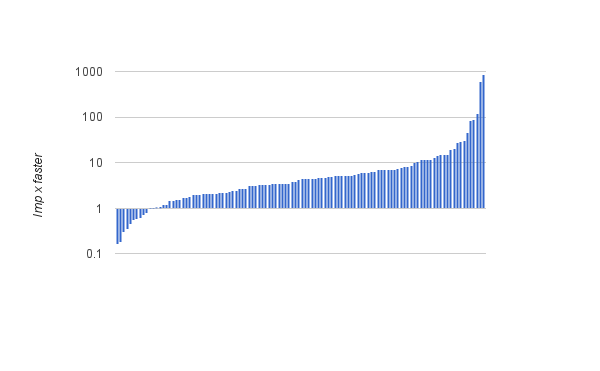
The vast majority of queries are between 10x slower and 10x faster, putting Imp squarely in the 'fast enough' range.
There are a few outliers where Imp is up to 867x faster. The worst of them is 29a, whose plan underestimates the number of rows by 4890x. Despite their claims to innocence, it's pretty clear the author deliberately crafted this query to confuse Postgres with cross-constraint correlations. While many of the queries contain correlations that might realistically come up (eg company.country_code = '[jp]' and name.name like '%Yu%') but the worst outliers have silly redundant constraints (eg title.title = 'Shrek 2' and keyword.keyword = 'computer-animation').
Memory usage for Imp during the benchmarks is around 16GB. The dataset is only 3.7GB on disk and overhead of the indexes doesn't account for more than a few GB. I haven't run a memory profiler yet, but I suspect it's caused by string allocation overhead and memory fragmentation (Julia doesn't have a compacting collector). The natural way to fix this would be to concatenate each column into a single string and store an array of indexes into that string, but boxing rears its ugly head again when we try to return substrings. A problem for another day.
What's missing from this experiment is an understanding of how the different design choices contribute to the results. It seems likely that Imp has a large constant-factor performance advantage due to the lack of IO and concurrency overheads. It also seems likely that I'm undoing most of that advantage by choosing sub-optimal plans. But without a more controlled experiment it's just speculation. A useful follow-up would be to extract variable orderings from LogicBlox, which uses the same join algorithm, and run them in Imp to see how much performance a commercial-quality planner buys.
Conclusion
There are three things that I think are worth taking away from this experiment:
-
Julia is almost a fantastic language for generative programming. The combination of a dynamic language, multiple dispatch, quasi-quoting, macros, eval and generated functions with predictable type-inference and specialization is killer. But in almost every part of Imp there was an elegant, efficient, extensible design that would work if the support for unboxing was as complete as the Julia team wants it to be. It's so nearly there.
-
The recent wave of worst-case-optimal join algorithms are really easy to implement with code generation and this lowers the bar for writing a query compiler. LegoBase and co already demonstrated the power of staging, but if you don't already have a fancy staging compiler for your favorite language you don't have to wait - Imp's query compiler could be directly translated into pretty much any language, either as a macro or as a preprocessor pass.
-
Automatic query planning might not be essential for every use-case. It certainly makes sense for interactive usage, and for cases where you are splicing user input into a query. But in cases where the queries are fixed and you have a rough idea of what the data looks like, it's possible to gain many of the benefits of a query compiler without the opacity of a full query planner.
Thanks to Lindsey Kuper and Joe Edelman for comments, and to Michael Malis for advice on tuning Postgres.