https://smile.amazon.com/dp/1482253445
Focuses on practical elements of modeling. Very skimpy on the math, but can get that elsewhere. Most of the value is in working through the exercises.
Book focuses on Bayesian data analysis, multilevel modeling and model comparison using information criteria.
Hypothesis <-> model <-> data are many-many relationships. Naive falsification is a myth - multiple hypotheses might have models which predict the same data, and one hypothesis might have multiple models that each predict different data. Worse, most interesting hypotheses are probabilistic. Eg 80% of swans are white - how many black swans do we have to see to falsify? How many blurry photos of Nessie do we have to see to falsify the no-Nessie hypothesis?
(NHST is not even naive falsification - it attempts to falsify the null hypothesis rather than the hypothesis in question. In many domains there is not even an obvious neutral hypothesis.)
Clearly need to be able to reason about evidence/belief/confidence. Bayesian approach is defined by using probability for both observed frequencies and evidence/belief/confidence. See Jaynes for the canonical argument that probability is the right way to think about belief.
No free lunch. Bayesian inference always takes place within some model. Within the assumptions of the model being fitted, Bayesian inference is optimal. BUT IT CANNOT TELL YOU IF YOUR MODEL IS CORRECT. Small world vs large world.
Cute metaphor of statistical modeling tools as golems - immensely powerful but brutally unthinking. User is responsible for supplying all the wisdom and interpretation.
Bayesian model consists of:
- Set of parameters
- Prior distribution on parameters
- Model mapping parameters to distribution on observed evidence
Epistemological assumption - about how to model the world. Ontological assumption - about the world. Projection fallacy - confusing the two. Eg model of height assumes that individual heights are IID. Not true for eg twins, but true enough to make the model useful.
Multilevel models - models where parameters are themselves supplied by models. Typical reasons for use:
- To adjust estimates for imbalanced / biased samples
- To study variation between subjects
- To avoid averaging over samples
The distinction only seems to need stating because the history of the subject focuses on single-level models.
Information criteria are used to estimate prediction performance across different models. Still no free lunch - each criteria embodies some set of assumptions about prediction. But useful for detecting overfitting, and for comparing multiple non-null models.
Book introduces three methods for conditioning on evidence:
- Grid approximation: approximate parameters by a discrete distribution on regular grid, compute discrete posterior directly
- Quadratic approximation: under reasonable assumptions the posterior is approximately Gaussian, so use hill-climbing to find peak (mean) and use numerical methods to approximate curvature near peak (variance).
- Markov chain Monte Carlo: construct a Markov chain whose steady-state distribution is the posterior, sample repeatedly to approximate.
Simulate posterior for:
- Model checking - see if the implied predictions make sense eg look at various summary statistics to check assumptions eg run lengths in assumed IID samples.
- Software validation - simulate some known model and then fit it again to see if we can recover the orginal parameters.
- Research design - simulate hypothesis to see if the proposed experiment will be effective (includes power analysis).
- Forecasting - use model to make new predictions, for application or for testing the model out-of-sample.
Modeling
Often useful to standardize input data into $\text{mean} + x * \text{stddev}$. Makes the resulting parameters easier to compare directly to each other. For large inputs, may avoid loss of precision. In linear models, removes the strong correlation between intercept and slope.
Recommends preprocessing data for polynomials, without justification eg d$weight.s2 <- d$weight.s^2.
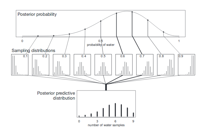
Posterior predictive distribution - sample from both posterior and model to compute prediction. Could compute it analytically, but we invented computers for this sort of thing.
Percentile intervals - what range of parameters occupies central X% of mass. Highest posterior density interval - what is the smallest range of parameters that covers X% of mass. Usually similar. If they aren’t, the distribution is weird and you should show the whole thing instead of summarizing it anyway.
What if we need a point estimate? Choose a loss function appropriate to your decision problem, and choose the point estimate that minimizes expected loss under the posterior distribution.
MAP estimate - maximum a posteriori - parameter with highest density in posterior.
Can display model uncertainty by sampling from the posterior and plotting the implied model eg for simple linear model plot the lines for each posterior sample.
Residual - difference between observation and prediction.
With multiple predictors, can no longer visualize predictions directly with a line + hpdi. Can use:
- Predictor residual plots - use all but one predictor to model remaining predictor, then regress+plot residuals against outcome. Shows the unique contribution of that predictor.
- Counterfactual plots - simulate altering one variable while holding the others constant.
- Posterior prediction plots - simulate and plot predicted outcome vs observed outcome, prediction error vs predictors, distribution of prediction error per case etc. In prediction error vs predictors, if the model is accurate we expect to see error distributed like the error term in our model. Obvious patterns are an opportunity for a better model.
Non-identifiability - when data and model structure do not allow estimating the value of a parameter.
Post-treatment bias - any variable that is a causal consequence of the treatment being studied can screen off the inferred influence of the treatment. Model is asking the wrong question, so model comparison using information criteria or out-of-sample prediction quality can’t help.
Linear models
Model outcome as linear function of predictors plus Gaussian error.
Why Gaussian? Gaussian distribution can originate from sum of similar-sized random variables or product of variables close to one ($(1+x)(1+y) \approx 1+x+y$), log of product of variables etc. Also Gaussian is lowest entropy distribution if all we know is mean and variance.
Handle categorical variables by separating into indicator variables.
Posterior for variance parameter tends to have a long right tail, because we know it’s non-negative. This makes the quadratic approximation suspect. Better to estimate $\log{\sigma}$ instead, which is closer to Gaussian. In general, using exponentials to constrain parameters to be positive, rather than using a one-sided prior, is a useful trick.
Can use multivariate linear regression to ‘control’ for effects of multiple variables.
Multicollinearity - when two predictor variables are strongly correlated, any linear combination of them will be equally plausible. Symptom is large spread and high covariance between posteriors for the two variables. (Special case of non-identifiability).
Polynomial regression - model outcome as polynomial of predictors plus Gaussian error. Not generally a good choice - hard to interpret and prone to overfitting. Better to start from a hypothesized mechanism.
Model comparison
Can’t judge significance by looking at marginal distributions of posterior - may be strong correlations between parameters. Eg may find that two parameters may both be centered around 0, but making one small makes the other large and vice versa. Safer to compare model with and model without parameter.
I found this section really hard to follow. Eventually realized that it’s notational sloppiness - not clearly distinguishing between expectations under reality and expectations under observation, and lack of clear indices on sums. These notes are heavily supplemented by other sources.
Under- vs over-fitting.
Regularization - use strong priors to penalize models which we believe are unlikely. Reduces over-fitting.
Cross-validation - partition the data into training and test set. Test how sensitive the parameters are to the partitioning.
For prediction tasks we can just choose models based on some cost function that matches the task. For scientific work we care about the model itself, so there is no clear cost function. KL-divergence from reality is a popular measure. The use of KL-divergence is really poorly justified in this text.
$D_{KL}(p,q) - D_{KL}(p,r) = E_p[\log(r) - \log(q)]$. We know $r$ and $q$ and we can approximate $E_p[\cdot]$ by averaging over the observed data, so we can easily estimate the difference in divergence between two models.
Minimizing KL-divergence is equivalent to maximizing the likelihood of the posterior over the observed data. Define deviance as $D(q) = -2 \sum_i \log(q_i)$ (summing over data). Roughly speaking, deviance : divergence as mean : expectation.
Now we want to estimate out-of-sample deviance. Various different estimators making different assumptions:
Akaike Information Criterion. $AIC = D(E_\theta[\theta]) + 2p$. Assuming flat priors, Gaussian posterior and sample size N » parameters k.
Deviance Information Criterion. $DIC = D(E_\theta[\theta]) + 2p_{DIC}$ where $p_{DIC} = E_\theta[D(\theta)] - D(E_\theta[\theta])$. Similar to AIC, but takes into account the fact that priors constrain degrees of freedom. Still assumes Gaussian posterior.
Widely Applicable Information Criterion. $WAIC = -2\text{lppd} - 2p_{WAIC}$ where $\text{lppd} = \sum_{i=1}^N \log E_\theta[P(y_i\vert\theta)]$ and $p_{WAIC} = \sum_{i=1}^N \text{Var}_\theta(\log P(y_i\vert\theta))$. Truely Bayesian calculation of deviance. Penalizes data points which have been fitted into a narrow peak. Assumes independent observations and that $p \ll N$.
Bayesian Information Criterion. Can be heavily influenced by choice of prior - not recommended.
Prefer WAIC where applicable, cross-validation otherwise.
Uniformitarian assumption - future data are expected to come from the same process as past data, with a similar range of hidden parameters. Pretty hard to avoid. Induction problem, basically.
Comparing models using information criteria only makes sense if both models are trained on the same data. Beware code that automatically drops missing data.
Akaike weight - map WAIC to probability scale, normalize across models. Use to compare relative accuracy. No consensus on how to interpret these weights - Akaike says:
A model’s weight is an estimate of the probability that the model will make the best predictions on new data, conditional on the set of models considered.
Model averaging - create an ensemble by summing Akaike weighted posteriors.
With enough model generation and comparison, we can overfit again.
Interactions
For linear interactions, multiply predictors together in the model.
Interactions are symmetric, so be sure to consider both interpretations.
Really hard to interpret, so definitely have to plot predictions now. Can use multiple plots to view interaction effects - varying predictor A across plots and predictor B within plots.
Centering data also becomes more important.
MCMC
Vague descriptions of how various MCMC algorithms work:
- Gibbs sampling. Something something conjugate pairs. Imposes limits on which priors you can pick. Inefficient when number of parameters grows to hundreds or thousands.
- Hamiltonian Monte Carlo. Uses derivatives to spend more time sampling regions with high curvature - when curvature is low we can just approximate by a plane. Requires continuous parameters. Requires tuning hyper-parameters but mostly automatable in practice.
Rule of thumb - use four-ish short chains to check that fitting is well-behaved, then use one long chain for actual inference.
Check that traces are stationary (same distribution over time) and well mixed (low correlation between adjacent points, no obvious patterns). Check that the estimated number of effective samples is high and that the potential scale reduction factor $\hat{R}$ converges to 1 (> 1.01 is suspicious).
Also simulate data from the model and check that inference recovers the original parameters.
Common failure modes:
- Broad flat regions in posterior (often caused by flat priors). Causes erratic jumps to extreme values.
- Non-identifiable parameters. Causes wandering traces.
Both are usually fixed by adding weakly informative priors.
Entropy
When choosing priors and likelihood functions, prefer the distribution with the maximum entropy that fits the constraints. Because:
- It adds the least additional information - can interpret this as making the fewest additional assumptions.
- Many natural process produce maximum entropy distributions eg mean of IID variables.
- It tends to work well in practice.
Wikipedias explanation of the Wallis derivation was easier to understand than the book.
Bayesian updates can be seen as a special case of minimizing cross entropy. Using the maximum entropy principle to justify minimizing cross-entropy is linguistically confusing. Think of it as minimizing information gain in both cases?.
Found a paper with the derivation but I couldn’t follow the notation after (32), so I worked through a really simple example instead:
Suppose we have a biased coin and we believe the bias $\theta$ is one of ${\frac{0}{3},\frac{1}{3},\frac{2}{3},\frac{1}{3}}$ with equal probability. Then we toss the coin and get heads. All we know about the new joint distribution $P_\mathrm{new}(\theta, X)$ is that $P_\mathrm{new}(\theta, X=\mathrm{Tails}) = 0$. The distribution that minimizes $D_\mathrm{KL}(P_\mathrm{new}, P_\mathrm{old})$ subject to that constraint is $P_\mathrm{new}(\theta, X = \mathrm{Heads}) = (\frac{0}{6}, \frac{1}{6}, \frac{2}{6}, \frac{3}{6})$ which is the same as we get from Bayes rule.
Maximum entropy distributions given:
- Fixed variance - Gaussian
- Positive, fixed mean - exponential
- Discrete, finite, fixed mean - binomial
- Discrete, fixed mean - geometric
Histomancy - trying to choose distribution by looking at histograms of data. Doesn’t work because distribution is for the residuals after the linear model and link function - can’t see it in the original data.
Generalized Linear Models
To use other distributions in a linear model we need to map the range of the linear model to the domain of the distribution parameters with a link function.
Logistic regression:
\begin{align} y_i & \sim \operatorname{Binomial}(1, p_i) \cr \log{\frac{p_i}{1-p_i}} & = \alpha + \beta x_i && (\text{logit}) \end{align}
Aggregated binomial regression:
\begin{align} y_i & \sim \operatorname{Binomial}(n_i, p_i) \cr \log{\frac{p_i}{1-p_i}} & = \alpha + \beta x_i \end{align}
(To use WAIC, we need to disaggregate the aggregated binomial model to get individual points.)
Poisson regression:
\begin{align} y_i & \sim \operatorname{Poisson}(\lambda_i) \cr \log{\lambda_i} & = \alpha + \beta x_i \end{align}
If the measurement periods for each case differ, can separate $\lambda_i = \mu_i / \tau_i$:
\begin{align} y_i & \sim \operatorname{Poisson}(\mu_i) \cr \log{\mu_i} & = \log{\tau_i} + \alpha + \beta x_i \end{align}
Deal with multiple outcome events either by normalizing multiple weights:
\begin{align} y_i & \sim \operatorname{Multinomial}(n_i, p) \cr p_i & = \frac{\exp{s_i}}{\sum_j \exp{s_j}} \cr s_1 & = \alpha + \beta x_i \cr s_2 & = \gamma y_i + \delta z_i \cr s_3 & = \text{etc…} \end{align}
Or by using multiple Poisson processes:
\begin{align} y_i & \sim \operatorname{Poisson}(\lambda_i) \cr \log{\lambda_1} & = \alpha + \beta x_i \cr \log{\lambda_2} & = \gamma y_i + \delta z_i \cr \log{\lambda_3} & = \text{etc…} \end{align}
(Presumably when total counts vary across cases, we should separate $\lambda_i = \mu_i / \tau_i$ again?)
Use sensitivity analysis to understand how choice of distribution and link function affect the results.
Beware - information criterion can’t compare models with different distributions, because the constant part of the deviance no longer cancels out in the difference.
Mixtures
Use multiple distributions to model a mixture of causes.
Ordered categorical model. Ordered categories such as ratings can’t be treated just like counts because they may produce non-linear effects eg moving a rating from 1/5 to 2/5 may be a bigger change than moving from 3/5 to 4/5.
\begin{align} y_i & \sim \operatorname{Ordered}(p_i) && \text{where $p_{i,k} = \operatorname{Pr}(y_i \le k)$} \cr \log{\frac{p_{i,k}}{1-p_{i,k}}} & = \alpha_k - \phi_i \cr \phi_i & = \beta_A A_i + \beta_I I_i + \beta_C C_i \cr \end{align}
I think the idea here is that the $\alpha_k$ map the ratings onto a linear scale and then variation in each case is modeled by $\phi_i$. Not confident though.
Zero-inflated models. Sometimes there are multiple ways to get 0 eg maybe there really were no bacteria in this sample, or maybe we screwed up and sterilized it while inspecting it.
Over-dispersion - when variance is higher than expected in the model results. May indicate missing predictors. Common strategies to deal with it include using a continuous mixture model or using multi-level models.
Beta-binomial model - a continuous mixture model that estimates a different binomial parameter for each case. (Uses a beta distribution because there is a closed form solution for the likelihood function.)
\begin{align} y_i & \sim \operatorname{Binomial}(n_i, \operatorname{Beta}(p_i, \theta))) \cr \operatorname{logit}(p_i) & = \beta_A A_i + \beta_I I_i + \beta_C C_i \cr \end{align}
Negative-binomial / gamma-poisson model - a continuous mixture model that estimates a different poisson parameter for each case. (Uses a gamma distribution, again, to make the math easy).
\begin{align} y_i & \sim \operatorname{Poisson}(\operatorname{Gamma}(\mu_i, \theta))) \cr \log(\mu_i) & = \beta_A A_i + \beta_I I_i + \beta_C C_i \cr \end{align}
(Beta-binomial and negative-binomial effectively add a hidden parameter per case, so can’t be aggregated or disaggregated without changing the structure of the inference which means they can’t be compared with WAIC.)
Multilevel models
Want to pool information between different groups, but only to the extent that the groups appear to be similar. So instead of inferring parameters independently for each group, model those parameters as being drawn from a common distribution.
Eg single level:
\begin{align} s_i & \sim \operatorname{Binomial}(n_i, p_i) \cr \operatorname{logit}(p_i) & = \alpha_{\mathrm{TANK}[i]} \cr \alpha_{\mathrm{TANK}} & \sim \operatorname{Normal}(0,5) \cr \end{align}
Eg multilevel:
\begin{align} s_i & \sim \operatorname{Binomial}(n_i, p_i) \cr \operatorname{logit}(p_i) & = \alpha_{\mathrm{TANK}[i]} \cr \alpha_{\mathrm{TANK}} & \sim \operatorname{Normal}(\alpha,\sigma) \cr \alpha & \sim \operatorname{Normal}(0,1) \cr \sigma & \sim \operatorname{HalfCauchy}(0,1) \cr \end{align}
The higher level prior can end up much more strongly regularizing than one the user would set by hand, in which case the lower level estimates will tend to shrink towards the mean and the effective number of parameters in WAIC will be lower than the single level model.
Can think of this as an adaptive tradeoff between complete pooling (ignore groups, treat all cases the same) and zero pooling (infer parameters for each group independently). In small groups, zero pooling risks overfitting. In large groups, complete pooling wastes valuable information. Partial pooling with a multilevel model smoothly trades off between the two across varying group sizes.
Any batch of parameters with exchangeable index values can and probably should be pooled. (Exchangeable just means the index values have no true ordering, because they are arbitrary labels.)
Covariance
Varying effects model. Can pool both intercepts and slopes in typical linear model. But intercepts and slopes might also covary, so rather than generating them separately we can model the covariance by drawing them from a joint distribution.
\begin{align} W_i & \sim \operatorname{Normal}(\mu_i, \sigma) \cr \mu_i & = \alpha_{\operatorname{CAFE}[i]} + \beta_{\operatorname{CAFE}[i]} A_i \cr \begin{bmatrix} \alpha_{\mathrm{CAFE}} \cr \beta_{\mathrm{CAFE}} \end{bmatrix} & \sim \operatorname{MVNormal}(\begin{bmatrix} \alpha \cr \beta \end{bmatrix}, S) \cr S & = \begin{pmatrix} \sigma_\alpha & 0 \cr 0 & \sigma_\beta \end{pmatrix} R \begin{pmatrix} \sigma_\alpha & 0 \cr 0 & \sigma_\beta \end{pmatrix} \cr \alpha & \sim \operatorname{Normal}(0, 10) \cr \beta & \sim \operatorname{Normal}(0, 10) \cr \sigma & \sim \operatorname{HalfCauchy}(0, 1) \cr \sigma_\alpha & \sim \operatorname{HalfCauchy}(0, 1) \cr \sigma_\beta & \sim \operatorname{HalfCauchy}(0, 1) \cr R & \sim \operatorname{LKJcorr(2)} \cr \end{align}
(Where $\operatorname{LKJcorr(\eta)}$ at $\eta = 1$ is a flat prior over all valid correlation matrices and at $\eta > 1$ is increasingly skeptical about strong correlations.)
Non-centered parameterization - use adaptive priors that express only correlation, not covariance, and use linear model to rescale. Otherwise many HMC engines struggle with varying effects models.
Gaussian process regression - handle continuous categories by building the covariance matrix from the distances between cases.
\begin{align} T_i & \sim \operatorname{Poisson}(\lambda_i) \cr \log{\lambda_i} & = \alpha + \gamma_{\operatorname{SOCIETY}[i]} + \beta_P \log{P_i} \cr \gamma & \sim \operatorname{MVNormal}(0, K) \cr K_{ij} & = \eta^2 \exp(- \rho^2 D_{ij}^2) + \delta_{ij} \sigma^2\cr \alpha & \sim \operatorname{Normal}(0, 10) \cr \beta_P & \sim \operatorname{Normal}(0, 1) \cr \eta^2 & \sim \operatorname{HalfCauchy}(0, 1) \cr \rho^2 & \sim \operatorname{HalfCauchy}(0, 1) \cr \sigma^2 & \sim \operatorname{HalfCauchy}(0, 1) \cr \end{align}
(Where $D_{ij}$ is the distance matrix, $\rho$ governs the decline of correlation as distance increases, $\eta$ determines the maximum covariance between groups and $\sigma$ describes covariation between multiple observations from the same group.)
Measurement error and missing data
Measurement error can be modeled directly.
Imputation - filling in missing data.
Missing Completely At Random imputation - assume missing fields are selected uniformly at random. Generative model pulls exact values from data where they exist and puts in a generic variable otherwise.
Thoughts
The combination of arbitrary generative models and model comparison makes far more sense to me than significance testing, which I never really wrapped my head around.
I still don’t know how to use Stan. I don’t think the wrapper library in this book worked in my favor. Using R is a pain too. Maybe I should try out PyMC3.